The Mathematics of World Cup Prediction Markets: How to Calculate True Edge Over the Crowd

Most people trading World Cup prediction markets on Polymarket treat contract prices as gospel. Spain is trading at 16.5 cents. France sits at 16.1 cents. England hovers near 10.9 cents. Traders glance at these numbers, decide whether they feel right, and click buy. They are leaving money on the table.

The $2 billion in volume flowing through Polymarket’s World Cup Winner market represents the single largest prediction market event in history. Yet the vast majority of that volume comes from traders who have never calculated an expected value, never stripped the vig from a multi-outcome market, and never sized a position using anything more sophisticated than gut instinct. The math that separates profitable traders from expensive spectators is approachable. It just requires actually doing it.

This article walks through every calculation you need: converting raw contract prices into implied probabilities, identifying and removing the overround baked into multi-outcome markets, computing expected value on individual positions, sizing those positions with the Kelly criterion, and spotting cross-platform arbitrage between Polymarket and Kalshi.

Every formula uses real prices pulled from live World Cup 2026 markets. By the end, you will have a complete mathematical framework for finding genuine edge in prediction markets, applicable well beyond this tournament.

Contract Prices and Implied Probability: The Foundation

Polymarket’s mechanics are simple at the surface level. Every outcome token is priced between $0.00 and $1.00. If an outcome happens, YES shares resolve to $1.00. If it doesn’t, they resolve to $0.00. The price, therefore, maps directly to the market’s implied probability for that outcome.

The conversion formula:

So if Spain YES shares trade at $0.165, the market collectively prices Spain’s probability of winning the 2026 World Cup at 16.5%.

Here are the live Polymarket prices for the top contenders in the World Cup Winner market as of early June 2026:

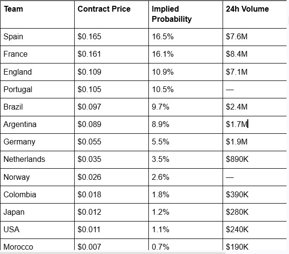
This looks straightforward. But there’s a problem hiding in these numbers that most traders never notice.

The Overround Problem: Why the Prices Lie

In a mathematically fair market, the probabilities of all mutually exclusive outcomes must sum to exactly 100%. Only one team can win the World Cup. The probabilities should add up to 1.00.

They don’t.

Add up every outcome’s price in the Polymarket World Cup Winner market (all 48 teams plus “Other” outcomes), and the total exceeds $1.00. The sum typically lands somewhere between $1.05 and $1.12 for major multi-outcome markets.

Let’s work through this with a smaller, more tractable example first. Polymarket’s Group F Second Place market has just four outcomes. As of early June 2026:

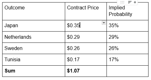
That $1.07 total is the overround. The excess above $1.00 is the market’s built-in margin: 7 percentage points of probability that doesn’t correspond to any real-world outcome. In traditional sports betting, this is called the vig, juice, or vigorish. On Polymarket, it emerges organically from the bid-ask spread in the CLOB (Central Limit Order Book) rather than being set by a bookmaker, but the mathematical effect is identical.

The overround means every price you see is inflated. You are overpaying relative to what the market actually believes, because the raw prices include a hidden tax distributed across all outcomes.

This matters enormously when you’re trying to find edge. If you think Japan’s true probability of finishing second in Group F is 36%, and the market shows 35%, you might think you’ve found a 1-percentage-point edge. But once you strip the vig, the market’s actual estimate of Japan’s probability is lower than 35%. Your edge might be larger than you think, or an apparent edge on another outcome might vanish entirely.

Stripping the Vig: The Normalization Method

The standard approach to removing overround is multiplicative normalization. You divide each outcome’s implied probability by the sum of all implied probabilities. This scales everything down proportionally so the total reaches exactly 100%.

The formula:

Let’s apply this to Group F Second Place:

Total Implied Probability (Σ) = 1.07

Verification: 32.71% + 27.10% + 24.30% + 15.89% = 100.00% ✓

The differences matter. Japan’s raw price implies 35%, but the market’s vig-adjusted belief is 32.71%. That’s a 2.29 percentage point gap. If your independent model says Japan has a 34% chance, your edge over the market’s true estimate is 1.29 points, not the negative 1 point you’d calculate from raw prices.

Now let’s apply this to the main World Cup Winner market. Taking the top 14 teams listed above plus a catch-all “Others” bucket at approximately 3 cents:

Σ = 0.165 + 0.161 + 0.109 + 0.105 + 0.097 + 0.089 + 0.055 + 0.035 + 0.026 + 0.018 + 0.012 + 0.011 + 0.007 + 0.005 + 0.105 (remaining ~36 teams combined) = ~1.10

With a 10% overround:

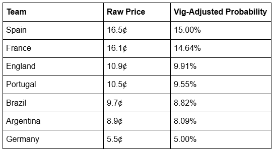
The gap between raw and adjusted is consistent percentage-wise but grows in absolute terms for the favorites. Spain’s raw price suggests 16.5%, but the market’s actual consensus probability is closer to 15.0% once you remove the overround. That 1.5 percentage points of phantom probability is money you’d be overpaying if you treated the raw price as the true probability.

Why Multiplicative Normalization Has Limits

Multiplicative normalization treats the overround as evenly distributed across all outcomes in proportion to their price. This assumption holds reasonably well when the overround is small (under 8–10%) and the market is liquid. But it breaks down in specific conditions.

The first problem: the favorite-longshot bias. Decades of sports betting research (Shin, 1991, 1993) show that bookmakers and markets systematically overprice longshots relative to favorites. In a 48-team tournament, the bulk of the overround often concentrates in the tails. Mexico at 0.5¢ and Morocco at 0.7¢ are probably more inflated, percentage-wise, than Spain at 16.5¢.

The Shin model accounts for this by assuming a fixed fraction (z) of informed traders in the market, which skews probability estimates toward favorites. The Shin-adjusted probability for outcome i is:

Where q(i) is the raw implied probability and z is the insider proportion parameter (typically estimated at 0.02 to 0.05 for liquid markets).

This gets computationally heavy fast with 48+ outcomes. For practical purposes in Polymarket’s World Cup markets, multiplicative normalization gives you a reasonable first approximation. The Shin correction matters most when you’re evaluating longshots (teams priced under 3 cents), where the favorite-longshot bias inflates prices the most.

The second problem: the bid-ask spread creates its own distortion layer. Polymarket’s displayed price is the midpoint of the bid-ask spread (or the last traded price if the spread exceeds $0.10). The actual execution price when buying is the ask, and when selling is the bid. This means your realized implied probability is different from the displayed implied probability, and we’ll address this separately below.

Expected Value: The Only Number That Matters

Once you have vig-adjusted probabilities, you can calculate expected value (EV) on any position. EV tells you whether a trade is profitable in the long run, regardless of whether any individual bet wins or loses.

The formula for a Polymarket YES position:

Or expressed as a percentage return:

Here’s where this gets concrete.

Worked Example 1: Spain to Win the World Cup

Polymarket asks $0.165 for Spain YES shares. The market’s vig-adjusted probability (using multiplicative normalization with a 10% overround) is 15.0%.

Suppose your own model, built on ELO ratings, squad depth analysis, group draw difficulty, and historical tournament performance, assigns Spain a 19% probability of winning the tournament.

For every dollar you deploy buying Spain YES shares at 16.5 cents, you expect to earn 15.15 cents in profit over the long run, given your probability estimate is accurate.

But notice the critical comparison. Your 19% estimate versus the vig-adjusted 15.0% gives you a 4 percentage point edge. If you had compared against the raw price (16.5%), you’d calculate only a 2.5 point edge. Stripping the vig revealed that your true edge is 60% larger than the naive calculation suggested.

Worked Example 2: Argentina to Win the World Cup

Argentina YES shares trade at $0.089. Vig-adjusted probability: 8.09%.

Your model gives Argentina a 7% chance. Lower than the market.

Negative EV. The market is pricing Argentina cheaper than the raw 8.9% suggests, but even at the vig-adjusted 8.09%, your model says they’re overpriced. This is a pass, or potentially a NO position.

For the NO side:

The NO side has positive expected value, but the return percentage is tiny: (0.93 / 0.911–1) × 100 = +2.09%. You’re tying up 91.1 cents per share to make 1.9 cents in expected profit. The capital efficiency is poor, which is why most prediction market traders focus on YES positions for underpriced outcomes rather than NO positions for overpriced ones.

Worked Example 3: A Group Stage Match

Polymarket’s USA vs. England match market (Group D):

OutcomePriceEngland Win$0.52Draw$0.20USA Win$0.28Sum: $0.52 + $0.20 + $0.28 = $1.00

Interesting. This is a three-way market that sums to exactly $1.00, meaning there’s zero overround in the displayed prices. This can happen in newer or less liquid Polymarket markets where the CLOB hasn’t generated enough spread yet. When the overround is zero, the displayed prices are the vig-adjusted probabilities. No correction needed.

But you still need to account for the bid-ask spread on execution, which we’ll cover shortly.

Your model says England has a 48% probability of winning this match. The market says 52%.

Negative EV. The market is overpricing England by 4 points according to your model.

What about a draw? Your model gives 24% for a draw, versus the market’s 20%.

That’s a 20% expected return. Draws are historically underpriced in football prediction markets because recreational bettors overwhelmingly bet on teams winning rather than draws. This pattern from traditional sportsbooks carries over into prediction markets like Polymarket.

The Kelly Criterion: How Much to Bet

Finding positive EV is only half the problem. The other half is how much of your bankroll to allocate. Bet too little and you leave profit on the table. Bet too much and a losing streak wipes you out before the edge pays off. The Kelly criterion solves this optimization problem precisely.

For a binary prediction market position (YES share that pays $1.00 or $0.00):

Where:

b = net payout per dollar risked = ($1.00 — Contract Price) / Contract Price

p = your estimated true probability

q = 1 — p

Worked Example: Kelly on Spain

Contract price: $0.165

Your probability: 19%

Kelly says to bet 2.99% of your bankroll on Spain at these prices and probabilities.

The Kelly fraction responds to two inputs: the size of your edge and the odds being offered. With World Cup outright markets offering long odds (5× to 200× payoffs), Kelly fractions tend to be small even with substantial edge. This is mathematically correct. Long-shot bets have high variance, and Kelly’s logarithmic utility function is conservative with high-variance positions.

Fractional Kelly

Most professional gamblers and traders use “fractional Kelly,” typically betting one-quarter to one-half of the full Kelly amount. The reasoning is straightforward: the Kelly criterion assumes your probability estimate is exactly correct. It never is. Estimation error means full Kelly consistently overbets in practice.

For our Spain example:

On a $10,000 bankroll:

Full Kelly: $299 on Spain

Half Kelly: $150 on Spain

Quarter Kelly: $75 on Spain

Quarter Kelly is the conservative professional standard. It sacrifices roughly 6% of the theoretical growth rate compared to full Kelly but reduces the maximum drawdown by about 50%.

Simultaneous Kelly Across Multiple Bets

The World Cup Winner market has 48 teams. You might identify positive EV on several of them simultaneously. The standard single-bet Kelly formula doesn’t account for the fact that these bets are mutually exclusive (if Spain wins, every other bet loses).

For mutually exclusive outcomes in a single market, the adjustment is:

This recursive relationship is computationally messy. A practical simplification: if your total Kelly allocation across all outcomes stays below 15–20% of your bankroll, the single-bet Kelly formula applied independently to each outcome gives a close approximation. The correlation adjustment only becomes material when you’re betting aggressively across many outcomes.

The Bid-Ask Spread: Your Hidden Cost

Everything above uses displayed midpoint prices. Actual execution prices are worse.

Polymarket uses a Central Limit Order Book where the displayed price is the midpoint between the best bid and best ask. If the best bid is $0.34 and the best ask is $0.40, the displayed price is $0.37. But when you buy, you pay $0.40. When you sell, you receive $0.34.

This spread functions as an additional transaction cost that directly reduces your expected value.

Let’s recalculate Spain with a realistic spread. The World Cup Winner market is extremely liquid ($380M in open liquidity), so the spread on top outcomes is tight. Suppose Spain shows:

```

Best Bid: $0.163

Best Ask: $0.167

Displayed Midpoint: $0.165

```

If you buy at the ask:

```

EV(buying at ask) = (0.19 × $1.00) — $0.167

EV = +$0.023 per share

EV% = (0.19 / 0.167–1) × 100 = +13.77%

```

Compared to +15.15% at the midpoint. The spread cost you 1.38 percentage points of expected return. In a market with $380 million in liquidity, that’s a modest cost. In thinner markets like Group F Second Place or individual player props, spreads can run $0.05 to $0.10 wide, eating half or more of a reasonable edge.

For any position you’re evaluating, always check the actual order book depth. A 5% edge calculated at midpoint can become a 0% edge at the ask.

Calculating Effective Vig from the Spread

In a two-outcome market (standard YES/NO), the bid-ask spread directly maps to the effective vig:

```

Effective Vig = (YES Ask + NO Ask) — $1.00

```

If YES Ask = $0.55 and NO Ask = $0.52:

```

Effective Vig = $0.55 + $0.52 — $1.00 = $0.07 = 7%

```

You can verify: anyone who buys both sides simultaneously pays $1.07 for shares that will collectively pay out $1.00 regardless of the outcome. That $0.07 loss is the market maker’s guaranteed profit (the vig).

In multi-outcome markets like the World Cup Winner, the calculation extends:

```

Effective Vig = Σ(Ask price for each outcome) — $1.00

```

If the sum of all ask prices across 48 teams equals $1.15, the effective vig for takers (market order buyers) is 15%. This is substantially higher than the midpoint-derived overround of 10% we calculated earlier. The difference is the market makers’ compensation for providing liquidity.

Cross-Platform Arbitrage: Polymarket vs. Kalshi

When the same event trades on multiple platforms at different prices, arbitrage opportunities appear. The 2026 World Cup trades actively on both Polymarket and Kalshi, with meaningful price discrepancies.

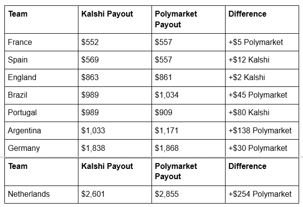
From Sports Illustrated’s comparison (late May 2026), the payout per $100 wagered on each platform:

Converting payouts back to implied probabilities (Implied Prob = $100 / Payout):

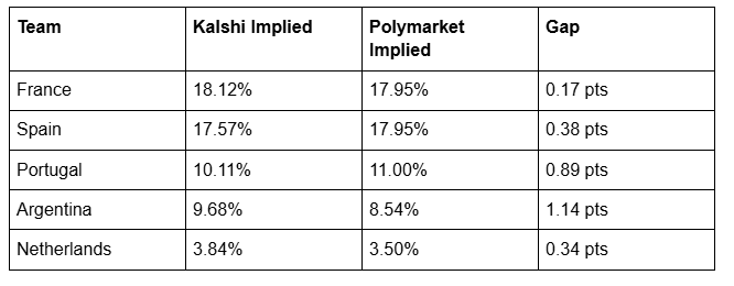
These cross-platform gaps represent theoretical edge for traders who can identify which platform’s price is “wrong.” The Portugal and Argentina discrepancies are the most actionable. Polymarket prices Portugal 0.89 points higher than Kalshi, while pricing Argentina 1.14 points lower than Kalshi.

True arbitrage (riskless profit) requires being able to buy YES on one platform and NO on the other simultaneously. In practice, capital requirements, withdrawal fees, and settlement timing make pure arbitrage difficult between a crypto-native platform (Polymarket) and a regulated US platform (Kalshi). But the price gaps inform directional conviction. If two independent markets with billions in combined volume disagree on Argentina by 1.14 points, at least one of them is wrong, and trading against the wrong one is positive EV.

Building Your Own Probability Model

All the math above assumes you have independent probability estimates. Where do those come from?

The baseline approach uses ELO ratings. FIFA’s own ranking system provides a starting point, but ELO-based models like FiveThirtyEight’s Soccer Power Index (now maintained by various successors), ClubELO, and World Football ELO give more statistically rigorous estimates. These models assign each team a rating based on historical match results, with adjustments for match importance, goal differential, and home-field advantage.

To convert ELO differences into match win probabilities:

```

Expected Score = 1 / (1 + 10^((ELO_B — ELO_A) / 400))

```

For example, if Spain has an ELO of 2050 and Cape Verde has an ELO of 1380:

```

Expected Score(Spain) = 1 / (1 + 10^((1380–2050)/400))

= 1 / (1 + 10^(-1.675))

= 1 / (1 + 0.0211)

= 1 / 1.0211

= 0.9793

```

Spain’s single-match win expectancy against Cape Verde: 97.93%.

Converting match-level probabilities to tournament-winner probabilities requires Monte Carlo simulation. You simulate the entire tournament bracket thousands of times (10,000+ iterations minimum), drawing match outcomes from your ELO-derived probabilities with random noise, and count how often each team wins the final. The fraction of simulations each team wins is your tournament probability.

A Python sketch of this process:

```python

import random

def simulate_match(elo_a, elo_b):

“””Returns 1 if team A wins, 0 if team B wins.”””

expected = 1 / (1 + 10**((elo_b — elo_a) / 400))

return 1 if random.random() < expected else 0

def simulate_tournament(team_elos, bracket, n_simulations=50000):

win_counts = {team: 0 for team in team_elos}

for in range(nsimulations):

# Simulate group stage, knockout rounds, final

winner = run_single_tournament(team_elos, bracket)

win_counts[winner] += 1

return {team: count/n_simulations for team, count in win_counts.items()}

```

The output gives you independent probability estimates to compare against Polymarket’s vig-adjusted prices. Where your Monte Carlo probability exceeds the market’s vig-adjusted probability, you have positive expected value.

Adjustments Beyond ELO

Raw ELO models miss several factors that matter in the World Cup specifically:

Squad fitness and injuries. The 2026 World Cup spans June 11 to July 19 across the United States, Canada, and Mexico. The compressed European club season ending in late May means several top squads will field fatigued or injured players. Your model should discount teams with confirmed absences in key positions.

Travel and climate. The tournament’s geographic spread across three countries and multiple climate zones creates heterogeneous conditions. Teams playing in Mexico City (elevation 2,240 meters) face altitude challenges that flatten ELO advantages. Teams from northern Europe playing afternoon matches in Houston or Miami in June face heat stress that historically reduces performance by 3–8% in measured metrics like distance covered.

Tournament experience coefficients. Teams with deep runs in recent World Cups and continental championships show 2–4% higher conversion rates in knockout stage matches compared to what ELO alone predicts. This “clutch” factor, while difficult to isolate causally, appears consistently in tournament data going back to 1998.

The 48-team expanded format itself. This is the first World Cup with 48 teams, 12 groups of 4, and a Round of 32 before the traditional knockout bracket. The extra knockout round means one additional elimination match for every team that advances past the group stage. Favorites face more opportunities to be upset.

Monte Carlo simulations consistently show that expanding from 32 to 48 teams reduces the tournament-win probability for top teams by 1.5 to 3 percentage points compared to a 32-team format, all else equal. If your model was calibrated on 32-team tournament data, you need to adjust downward for favorites.

A Complete Worked Example: Evaluating Germany

Let’s put the entire framework together for a single position evaluation.

Step 1: Gather the market data.

Germany YES shares: $0.055 (displayed midpoint)

Order book: Bid $0.053, Ask $0.057

Spread: $0.004 (tight, indicating good liquidity)

Overround (total market): ~110%

Step 2: Calculate vig-adjusted probability.

```

Vig-adjusted probability = 0.055 / 1.10 = 0.050 = 5.00%

```

The market’s true consensus probability for Germany winning the World Cup is approximately 5.0%.

Step 3: Build your independent estimate.

Germany’s ELO: ~2020

Group E opponents: Curaçao (ELO ~1200), Ecuador (ELO ~1680), Ivory Coast (ELO ~1560)

Group stage advancement probability (from Monte Carlo, 50,000 simulations): 94.2%

Germany is in Group E with no elite opponent. Group advancement is near-certain. But the knockout path starting from the Round of 32 adds five elimination matches before the final. Using ELO-adjusted match probabilities through a simulated bracket:

Your model’s tournament win probability for Germany: 6.8%

Step 4: Calculate expected value.

Using the ask price (what you’d actually pay):

```

EV = (0.068 × $1.00) — $0.057

EV = +$0.011 per share

EV% = (0.068 / 0.057–1) × 100 = +19.30%

```

Positive EV of 19.3%. Your model sees Germany as underpriced by 1.8 percentage points relative to the vig-adjusted market probability.

Step 5: Size the position with Kelly.

```

b = ($1.00 — $0.057) / $0.057 = $0.943 / $0.057 = 16.54

p = 0.068

q = 0.932

f* = (16.54 × 0.068–0.932) / 16.54

f* = (1.1247–0.932) / 16.54

f* = 0.1927 / 16.54

f* = 0.01165

```

Full Kelly: 1.165% of bankroll.

Quarter Kelly: 0.29% of bankroll.

On a $10,000 bankroll at quarter Kelly: $29 on Germany.

That feels small. It should feel small. Your edge is modest (1.8 percentage points), the odds are long (16.5×), and the Kelly criterion is correctly reflecting the high variance inherent in low-probability bets. Traders who bet more than Kelly on longshots are mathematically guaranteed to underperform over a large sample, regardless of how confident they feel about individual picks.

Step 6: Document and track.

Record your entry price, probability estimate, Kelly fraction, and the date. After the tournament, you can evaluate whether your probability estimates were well-calibrated across all positions, not whether individual bets won or lost. Calibration analysis, not outcome analysis, is how you improve a prediction market model.

Advanced: The Implied Probability Surface

Sophisticated prediction market traders don’t just evaluate individual outcomes. They look at the probability surface across related markets for internal consistency.

Polymarket runs 193+ World Cup markets: the tournament winner, 12 group winners, 104 match outcomes, and 28+ prop markets. These markets should be mathematically consistent with each other. If Spain’s tournament winner probability is 16.5%, that number should be derivable from Spain’s group advancement probability, multiplied by their conditional probability of winning each subsequent knockout match, through to the final.

When the probabilities across related markets are inconsistent, someone is mispricing something.

Here’s how to check. Polymarket’s Group of Champions market (which group the eventual winner comes from) shows:

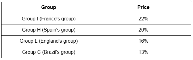
Group H contains Spain, Uruguay, Cape Verde, and Saudi Arabia. The group’s 20% chance of producing the champion should roughly equal Spain’s tournament probability plus Uruguay’s tournament probability (the other realistic contender in the group).

From the Winner market: Spain ~16.5%, Uruguay ~2%.

Sum: 18.5%

The Group of Champions market says 20%. The 1.5 point gap could reflect overround in both markets, or it could mean one market is slightly mispriced relative to the other. Cross-referencing like this across the full set of 193+ markets is where the deepest edges hide.

What This Math Actually Tells You

Running these calculations forces a specific kind of intellectual honesty. You cannot hide behind vague intuitions about which team “looks strong.” You have to assign a specific number, calculate whether that number implies profit at the current price, and decide exactly how much to bet based on how confident you are.

Most traders who go through this process for the first time discover two things. First, their edges are smaller than they assumed. A 2–3 percentage point edge on a 15% probability event feels like you know something the market doesn’t. In practice, it translates to modest expected returns with high variance. The math forces humility.

Second, the edges that exist tend to cluster in specific places. Group stage match markets (especially draws) are consistently underpriced relative to model-derived probabilities. Longshots beyond the top 8 teams tend to be overpriced due to recreational money and the favorite-longshot bias. Cross-platform gaps between Polymarket and Kalshi create structural opportunities when one platform’s user base reacts more slowly to news.

The math doesn’t make you a winner on any single trade. It makes you profitable over 50, 100, 500 trades, because you’re systematically identifying positions where the price is wrong, quantifying how wrong it is, and sizing your bets so that variance can’t destroy you before the edge pays off.

The $2 billion flowing through Polymarket’s World Cup markets is mostly guessing. The math is available to everyone. Almost nobody does it.